Title: Find a polynomial least squares fit for a set of points in C#

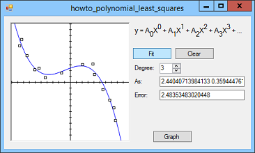
This example shows how to make a polynomial least squares fit to a set of data points. It's kind of confusing, but you can get through it if you take it one step at a time.

The example Find a linear least squares fit for a set of points in C# explains how to find a line that best fits a set of data points. If you haven't read that example yet, you should do so now because this example follows the same basic strategy.

With a degree d polynomial least squares fit, you need to find the coefficients A₀, A₁, ... A_d to make the following equation fit the data points as closely as possible:

    A0 * x0 + A1 * x1 + A2 * x2 + ... +  + Ad * xd

The goal is to minimize the sum of the squares of the vertical distances between the curve and the points.

Keep in mind that you know all of the points so, for given coefficients, you can easily loop through all of the points and calculate the error.

If you store the coefficients in a List<double>, then the following function calculates the value of the function F(x) at the point x.

// The function. public static double F(List<double> coeffs, double x) { double total = 0; double x_factor = 1; for (int i = 0; i < coeffs.Count; i++) { total += x_factor * coeffs[i]; x_factor *= x; } return total; }

The following function uses the function F to calculate the total error squared between the data points and the polynomial curve.

// Return the error squared. public static double ErrorSquared(List<PointF> points, List<double> coeffs) { double total = 0; foreach (PointF pt in points) { double dy = pt.Y - F(coeffs, pt.X); total += dy * dy; } return total; }

The following equation shows the error function:

To simplify this, let E_i be the error in the ith term so:

The steps for finding the best solution are the same as those for finding the best linear least squares solution:

• Take the partial derivatives of the error function with respect to the variables, in this case A₀, A₁, ... A_d.
• Set the partial derivatives equal to 0 to get N + 1 equations and N + 1 unknowns A₀, A₁, ... A_d.
• Solve the equations for A₀, A₁, ... A_d.

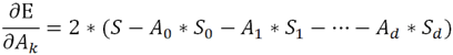
As was the case in the previous example, this may sound like an intimidating problem. Fortunately the partial derivatives of the error function are simpler than you might think because that function only involves simple powers of the As. For example, the partial derivative with respect to A_k is:

The partial derivative of E_i with respect to A_k contains lots of terms involving powers of x_i and different As, but with respect to A_k all of those are constants except the single term A_k * x_i^k. All of the other terms drop out leaving:

If you substitute the value of E_i, multiply the -x_i^k term through, and add the As separately you get:

As usual, this looks pretty messy, but if you look closely you'll see that most of the terms are values that you can calculate using the x_i and y_i values. For example, the first term is simply the sum of the products of the y_i values and the x_i values raised to the kth power. The next term is A₀ times the sum of the x_i values raised to the kth power. Because the y_i and x_i values are all known, this equation is the same as the following for a particular set of constants S:

This is a relatively simple equation with d + 1 unknowns A₀, A₁, ..., A_d.

When you take the partial derivatives for the other values of k as k varies from 0 to d, you get d + 1 equations with d + 1 unknowns, and you can solve for the unknowns.

Linear least squares is a specific case where d = 1 and it's easy to solve the equations. For the more general case, you need to use a more general method such as Gaussian elimination. For an explanation of Gaussian elimination, see Solve a system of equations with Gaussian elimination in C#.

The following code shows how the example program finds polynomial least squares coefficients.

// Find the least squares linear fit. public static List<double> FindPolynomialLeastSquaresFit( List<PointF> points, int degree) { // Allocate space for (degree + 1) equations with // (degree + 2) terms each (including the constant term). double[,] coeffs = new double[degree + 1, degree + 2]; // Calculate the coefficients for the equations. for (int j = 0; j <= degree; j++) { // Calculate the coefficients for the jth equation. // Calculate the constant term for this equation. coeffs[j, degree + 1] = 0; foreach (PointF pt in points) { coeffs[j, degree + 1] -= Math.Pow(pt.X, j) * pt.Y; } // Calculate the other coefficients. for (int a_sub = 0; a_sub <= degree; a_sub++) { // Calculate the dth coefficient. coeffs[j, a_sub] = 0; foreach (PointF pt in points) { coeffs[j, a_sub] -= Math.Pow(pt.X, a_sub + j); } } } // Solve the equations. double[] answer = GaussianElimination(coeffs); // Return the result converted into a List<double>. return answer.ToList<double>(); }

The code simply builds an array holding the coefficients (the Ss in the previous equation) and then calls the GaussianElimination method to find the As. It converts the result from an array into a List<double> for convenience and returns it.

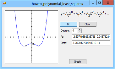
Give the program a try. It's pretty cool!

Tip: Use the smallest degree that makes sense for your problem. If you use a very high degree, the curve will fit the points very closely but it will probably emphasize structure that isn't really there. For example, the previous picture on the right fits a degree 4 polynomial to points that really should be fit with a degree 2 polynomial.

Download the example to experiment with it and to see additional details.